Dive into Neural Networks, the backbone of modern AI, understand its mathematics, implement it from scratch, and explore its applications

Neural networks are at the core of artificial intelligence (AI), fueling a variety of applications from spotting objects in photos to translating languages. In this article, we’ll dive into what neural networks are, how they work, and why they’re a big deal in our technology-driven world today.

1: Understanding the Basics

1.1: What are Neural Networks?

Neural networks are a cool blend of biology and computer science, inspired by our brain’s setup to tackle complicated computing tasks. Essentially, they’re algorithms designed to spot patterns and make sense of sensory data, which lets them do a ton of stuff like recognizing faces, understanding spoken words, making predictions, and understanding natural language.

The Biological Inspiration

Our brains have about 86 billion neurons, all linked up in a complex network. These neurons chat through connections called synapses, where signals can get stronger or weaker, influencing the message passed along. This is the foundation of how we learn and remember things.

Artificial neural networks take a page from this book, using digital neurons or nodes that connect in layers. You’ve got input layers that take in data, hidden layers that chew on this data, and output layers that spit out the result. As the network gets fed more data, it adjusts the connection strengths (or “weights”) to learn, kind of like how our brain’s synapses strengthen or weaken.

From Perceptrons to Deep Learning
Neural networks started with something called a perceptron in 1958, thanks to Frank Rosenblatt. This was a basic neural network meant for simple yes-or-no-type tasks. From there, we built more complex networks, like multi-layer perceptrons (MLPs), which can understand more complicated data relationships thanks to having one or more hidden layers.

Then came deep learning, which is all about neural networks with lots of layers. These deep neural networks are capable of learning from huge piles of data, and they’re behind a lot of the AI breakthroughs we hear about, from beating human Go players to powering self-driving cars.

Understanding Through Patterns
One of the biggest strengths of neural networks is their ability to learn patterns in data without being directly programmed for specific tasks. This process, called “training,” lets neural networks pick up on general trends and make predictions or decisions based on what they’ve learned.

Thanks to this capability, neural networks are super versatile and can be used for a wide array of applications, from image recognition to language translation, to forecasting stock market trends. They’re proving that tasks once thought to require human intelligence can now be tackled by AI.

1.2: Types of Neural Networks

Before diving into their structure and math, let’s take a look at the most popular types of Neural Networks we may find today. This will give us a better understanding of their potential and capabilities. I will try to cover all of them in future articles, so make sure to subscribe!

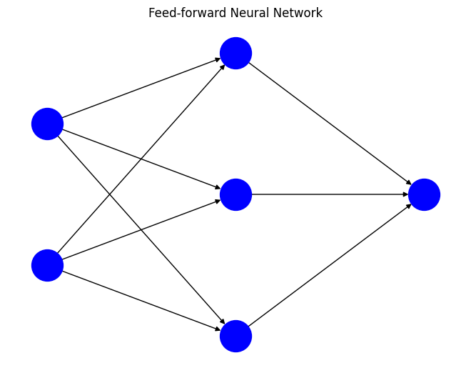
Feedforward Neural Networks (FNN)
Starting with the basics, the Feedforward Neural Network is the simplest type. It’s like a one-way street for data — information travels straight from the input, through any hidden layers, and out the other side to the output. These networks are the go-to for simple predictions and sorting things into categories.

Convolutional Neural Networks (CNN)
CNNs are the big guns in the world of computer vision. They’ve got a knack for picking up on the spatial patterns in images, thanks to their specialized layers. This ability makes them stars at recognizing images, spotting objects within them, and classifying what they see. They’re the reason your phone can tell a dog from a cat in photos.

Recurrent Neural Networks (RNN)
RNNs have a memory of sorts, making them great for anything involving sequences of data, like sentences, DNA sequences, handwriting, or stock market trends. They loop information back around, allowing them to remember previous inputs in the sequence. This makes them ace at tasks like predicting the next word in a sentence or understanding spoken language.

Long Short-Term Memory Networks (LSTM)
LSTMs are a special breed of RNNs built to remember things for longer stretches. They’re designed to solve the problem of RNNs forgetting stuff over long sequences. If you’re dealing with complex tasks that need to hold onto information for a long time, like translating paragraphs or predicting what happens next in a TV series, LSTMs are your go-to.

Generative Adversarial Networks (GAN)
Imagine two AIs in a cat-and-mouse game: one generates fake data (like images), and the other tries to catch what’s fake and what’s real. That’s a GAN. This setup allows GANs to create incredibly realistic images, music, text, and more. They’re the artists of the neural network world, generating new, realistic data from scratch.

2: The Architecture of Neural Networks

At the core of neural networks are what we call neurons or nodes, inspired by the nerve cells in our brains. These artificial neurons are the workhorses that handle the heavy lifting of receiving, crunching, and passing along information. Let’s dive into how these neurons are built.

2.1: The Structure of a Neuron

A neuron gets its input either directly from the data we’re interested in or from the outputs of other neurons. These inputs are like a list, with each item on the list representing a different characteristic of the data.

For each input, the neuron does a little math: it multiplies the input by a “weight” and then adds a “bias.” Think of weights as the neuron’s way of deciding how important an input is, and bias as a tweak to make sure the neuron’s output fits just right. During the network’s training, it adjusts these weights and biases to get better at its job.

Next, the neuron sums up all these weighted inputs and biases and runs the total through a special function called an activation function. This step is where the magic happens, allowing the neuron to tackle complex patterns by bending and stretching the data in nonlinear ways. Popular choices for this function are ReLU, Sigmoid, and Tanh, each with its way of tweaking the data.

2.2: Layers

Neural networks are structured in layers, sort of like a layered cake, with each layer made up of multiple neurons. The way these layers stack up forms the network’s architecture:

Input Layer
This is where the data enters the network. Each neuron here corresponds to one feature of the data. In the image above the input layer is the first layer on the left holding two nodes.

Hidden Layers
These are the layers sandwiched between the input and output, as we can see from the image above. You might have just one or a bunch of these hidden layers, doing the grunt work of computations and transformations. The more layers (and neurons in each layer) you have, the more intricate patterns the network can learn. But, this also means more computing power is needed and a higher chance of the network getting too caught up in the training data, a problem known as overfitting.

Output Layer
This is the network’s final stop, where it spits out the results. Depending on the task, like if it’s classifying data, this layer might have a neuron for each category, using something like the softmax function to give probabilities for each category. In the image above, the last layer holds only one node, suggesting that the is used for a regression task.

2.3: The Role of Layers in Learning

The hidden layers are the network’s feature detectives. As data moves through these layers, the network gets better at spotting and combining input features, layering them into a more complex understanding of the data.

With each layer the data passes through, the network can pick up on more intricate patterns. Early layers might learn basic stuff like shapes or textures, while deeper layers get the hang of more complex ideas, like recognizing objects or faces in pictures.

3: The Mathematics of Neural Networks

3.1: Weighted Sum

The first step in the neural computation process involves aggregating the inputs to a neuron, each multiplied by their respective weights, and then adding a bias term. This operation is known as the weighted sum or linear combination. Mathematically, it is expressed as:

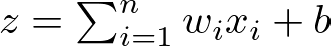
where:

• z is the weighted sum,
• wi​ represents the weight associated with the i-th input,
• xi​ is the i-th input to the neuron,
• b is the bias term, a unique parameter that allows adjusting the output along with the weighted sum.

The weighted sum is crucial because it constitutes the raw input signal to a neuron before any non-linear transformation. It allows the network to perform a linear transformation of the inputs, adjusting the importance (weight) of each input in the neuron’s output.

3.2: Activation Functions

As we said before, activation functions play a pivotal role in determining the output of a neural network. They are mathematical equations that determine whether a neuron should be activated or not. Activation functions introduce non-linear properties to the network, enabling it to learn complex data patterns and perform tasks beyond mere linear classification, which is essential for deep learning models. Here, we delve into several key types of activation functions and their significance:

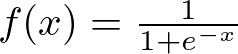
Sigmoid Activation Function

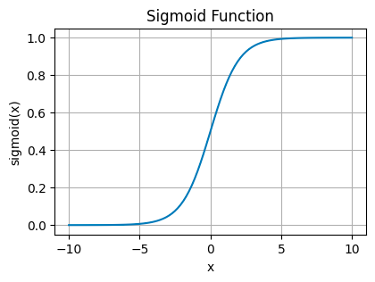
This function squeezes its input into a narrow range between 0 and 1. It’s like taking any value, no matter how large or small, and translating it into a probability.

You’ll see sigmoid functions in the final layer of binary classification networks, where you need to decide between two options — yes or no, true or false, 1 or 0.

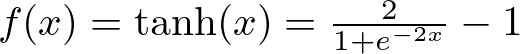
Hyperbolic Tangent Function (tanh)

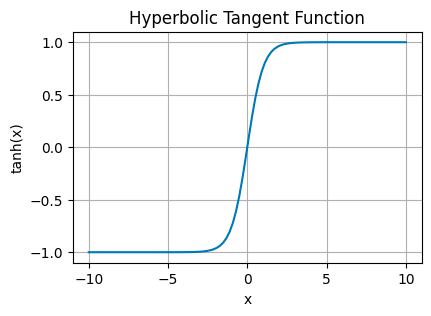
tanh stretches the output range to between -1 and 1. This centers the data around 0, making it easier for layers down the line to learn from it.

It’s often found in the hidden layers, helping to model more complex data relationships by balancing the input signal.

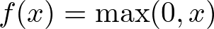
Rectified Linear Unit (ReLU)

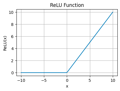
ReLU is like a gatekeeper that passes positive values unchanged but blocks negatives, turning them to zero. This simplicity makes it very efficient and helps overcome some tricky problems in training deep neural networks.

Its simplicity and efficiency have made ReLU incredibly popular, especially in convolutional neural networks (CNNs) and deep learning models.

Leaky Rectified Linear Unit (Leaky ReLU)

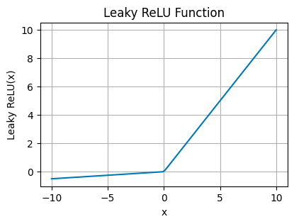
Leaky ReLU allows a tiny, non-zero gradient when the input is less than zero, which keeps neurons alive and kicking even when they’re not actively firing.